Description

Depression Detection Using Advanced Graphical Deep Learning – Part 4 (Graph Topology)

Introduction

Electroencephalography (EEG) is widely utilized in clinical settings for disease detection because of its high temporal resolution, non-invasiveness, and inexpensive data-gathering costs. Research in psychological and cognitive sciences has demonstrated that EEG signals can effectively reflect the majority of psychological and cognitive functioning. Prior research has utilized approaches such as dimensionality reduction or extraction of frequency band signals beforehand as features and subsequently applied machine learning algorithms as classifiers to carry out related tasks. However, the efficacy of these methods is highly dependent on the precision of the chosen features, and there is no connection between the classifier and the pre-extracted features.

Prior studies have aimed to utilize deep learning methods for analyzing EEG data in many applications, including emotion detection, motor imaging, and disease diagnosis. Several research efforts have endeavored to extract efficient biomarkers from EEG data in order to identify depression. Among the various approaches utilized, deep learning techniques can be roughly classified into two categories: CNN-based (Convolutional Neural Network) and GNN-based (Graph Neural Network).

CNN-based algorithms treat EEG data as images and utilize convolutional kernels to extract features. However, they do not fully take into account the interplay between multiple channels. In contrast, GNN-based algorithms transform EEG signals into data with a graph structure and utilize pre-computed graph adjacency matrices to depict the connections between various channels. These approaches consider the overall spatial structural linkages between different channels, making it easier to extract features that are connected across channels. Nevertheless, pre-calculated techniques are limited to producing unchanging adjacency matrices, which fail to capture the variations in individual brain networks and the dynamic alterations in network connections.

We present the concept of self-attention graph pooling and suggest a Graph Topology-based Max-Pooling (GTMP) module to improve it. Pooling layers are frequently employed in deep learning models to decrease the quantity of model parameters, promote computational efficiency, and raise the resilience of feature extraction. Nevertheless, the traditional pooling function is overly simplistic and fails to consider the abundant topological structural information that exists in the graph.

Unlike traditional pooling methods, we compute node relevance scores based on the structure of the graph and create a node mask. The representation vector of the graph is then determined by keeping the feature vector of the node with the greatest score.

Challenges

Current GNN-based algorithms continue to encounter difficulties. To begin with, there are differences in the brain networks among individuals, and the neural systems of the human brain are quite intricate. The existing methods are inadequate in precisely constructing comprehensive brain network topological structures, especially when it comes to mimicking the dynamic changes of the brain network. Furthermore, the current research has failed to incorporate the temporal dependency information of brain networks.

Diagnosing depression using Graph Neural Networks (GNN) usually requires pre-computing the adjacency matrix. However, this approach fails to include the differences in brain network connection between individuals with depression and those who are mentally well. In order to address this problem, we suggest implementing an Adaptive Network Topology Generation (AGTG) module. This module will create the connections between different elements of a network by analyzing EEG data in a flexible and adaptable manner.

Requirement of the Graph Topology

The AGTG module is important for building the topological connectivity of a graph with regard to the EEG signals adaptively. This flexibility helps guarantee that the structure of the graph reflects many-to-many relations between the areas of the human brain with great accuracy. Enhancing the accuracy of connectivity is another interesting goal of AGTG since it intends to combine distance, as well as the links between, various channels. This integration enables the model to take both the Euclidean distance between the brain regions and the functional connectivity into consideration, thereby making it possible to provide a more accurate picture of the brain’s connectivity than if the two were used individually.

As mentioned before, the AGTG module also has an adaptable structure, which enables it to modify the graph’s topology depending on the given features of the input EEG signals. Consequently, the structure of the graph that is obtained is adaptable to every person’s specific brain network characteristics, which in turn makes the diagnostic predictions more precise and accurate. In this process, AGTG lets the universal graph adjacency matrix and correlation matrix fix each other and acquire the final graph adjacency matrix, which displays the brain’s network connections in an optimal manner. This mutual correction mechanism helps to correct the topology of the graph as to the existing relationships between different brain regions and, therefore, increases the model’s diagnostic potential.

Process

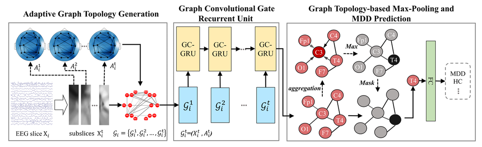
Adaptive Graph Topology Generation

The Adaptive Network Topology Generation (AGTG) module creates the connections between nodes in a network using EEG signals in a flexible way, namely by generating an adjacency matrix. The objective of our approach is to achieve enhanced connection that is both adaptable and accurate by combining spatial distance and correlations across several channels.

Initially, we present a universal graph adjacency matrix (A_{com}) that represents the overall connectivity state of brain networks based on distance. The calculation involves determining the spatial distance between different electrodes and expressing it in the following manner (eq-1).

A_com = {A | A_ij = norm(dis(i,j))}, (i,j = 1,2,…,E)

In the present scenario, the term norm refers to the normalization function, while dis(i,j) reflects the Euclidean distance between electrodes i and j based on the EEG electrode location. The symbol E represents the number of nodes in the network structure, specifically the number of EEG channels.

Afterwards, we perform a left multiplication of the matrix P on the input EEG signals X to capture the correlations across distinct channels. Then, we perform a right multiplication of the mapping matrix Q to translate these correlations onto an E-dimensional matrix called (A{cor}). The absolute value function is employed to capture the mutually exclusive or synchronous correlations between different channels and obtain the correlation matrix (A{cor}). This correlation matrix is expressed as follows (eq-2):

A_cor = abs(PXQ + b) (2)

In this particular instance, abs represents the absolute value function. The symbols P∈R and Q∈R refer to learnable parameter matrices, where F represents the feature dimension and ‘b’ represents the bias value.

Ultimately, we enable the universal graph adjacency matrix and the correlation matrix to reciprocally rectify one another in order to ascertain the ultimate graph adjacency matrix, which is specified by the following (eq-3):

A = Relu(A_cor + A_com * d) (3)

The variable d represents the weight parameter of the universal graph adjacency matrix that may be adjusted through learning. The Relu function is used to guarantee that all components in the matrix have values greater than or equal to zero.

Graph Topology-Based Max-Pooling and MDD Prediction

In order to improve the model’s performance, we propose the concept of self-attention graph pooling and develop a Graph Topology-based Max-Pooling (GTMP) module that takes into account both node characteristics and graph connectivity. This allows for the accurate extraction of graph representations.

Within this module, our initial task is to assess the importance of each individual node in the graph by analyzing the output (H_t) generated by the GCGRU module. It is presumed that if a node is engaged in the aggregation of features from multiple other nodes, it signifies a greater level of significance. Hence, we employ feature aggregation using the graph topological structure to calculate the significance score Snode for each node, according to the given phrase (eq-4).

S_node = Relu(AH_t W + b) (4)

The notation (H_t∈R) denotes the graph feature matrix generated by the GRU module, with ‘h’ representing the dimension of the hidden state. The matrix (A) is the laplacian matrix that has been symmetrically normalized. It corresponds to the graph feature (H_t). The matrices W and b represent the parameter matrix and bias value, respectively.

Afterwards, we arrange the nodes according to their significance scores and provide the indices of the top num nodes, which are represented by (N_{idx}).

Due to the utilization of max-pooling, the value of num is equal to 1. The term (N_{idx}) is defined in the following (eq-5):

N_idx = top-rank(S_node, num) (5)

The function top-rank() returns the indices of the num nodes with the highest scores.

Ultimately, we generate a node mask using the index of the node, (N_{idx}), and then use it to filter the graph feature matrix, (Ht). This process allows us to keep the most significant node feature vector as the graph representation vector, which we refer to as (V{graph}) (eq-6).

V_graph = mask(N_idx) ⨀ H_t(6)

The function mask() generates a mask vector by constructing it based on the node indices. Subsequently, the graph representation vector (V_{graph}), generated by the GTMP module, is fed into a fully connected layer to compute the likelihood of depression.

Code Description

The AGTG_Model class in Figure 1 depicts a graph transformation mechanism. These contain the initial value of ‘P’, ‘Q’, ‘b’, and ‘d’ in its constructor. The D_Matrix method computes the degree matrix ‘D’ of a graph from the adjacency matrix ‘A’ and gets the inverse square root of ‘D’. The forward method performs the graph transformation: after that, it then calculates a new adjacency matrix named A that can be computed through the ‘ReLU’ activation of the sum between the absolute value of ‘PXQ+b’ and the element-wise product between the original adjacency matrix and ‘d’. It then uses this new adjacency matrix ‘A’ to compute the degree matrix, to get a new matrix ‘A_norm’ which is returned as the output. The input here is the adjacency matrix and node features represented by ‘X’ and the goal of the model is to output a new graph which has updated values of edges’ weights. The change is driven by the learnable parameters and the initial graph along with adjacency information.

class AGTG_Model(nn.Module):
                def __init__(self, nodes_dim, node_features_dim):
                        super().__init__()
                        self.E = nodes_dim   # 
                        self.F = node_features_dim
                        self.P = nn.Parameter(torch.randn(self.E,self.E), requires_grad=True)
                        self.Q = nn.Parameter(torch.randn(self.F,self.E), requires_grad=True)
                        self.b = nn.Parameter(torch.randn(self.E,1), requires_grad=True)
                        self.d = nn.Parameter(torch.randn(1), requires_grad=True)

                def D_Matrix(self, A):
                         d = torch.sum(A, 1)
                         d_inv_sqrt = d**(-(1/2))
                         D_inv_sqrt = torch.diag(d_inv_sqrt)
                         return D_inv_sqrt

                def forward(self, X, adjacency_matrix):
                        I = torch.eye(self.E)
                        PX = torch.matmul(self.P, X)
                        PXQ = torch.matmul(PX, self.Q)
                        A_cor = torch.abs(PXQ+self.b)
                        A = nn.functional.relu(A_cor+adjacency_matrix*self.d)
                        A_I = A+I
                        D = self.D_Matrix(A_I)
                        A_norm = torch.matmul(D, torch.matmul(A_I, D))
                        return A_norm

Figure 1: Adaptive Graph Topology Generation Module

The GraphTopologyMaxPooling_Model class depicted in figure 2 defines a graph-based GRU model with max-pooling functionality. This also involves initializing parameters W, b, and ‘W_logit’ in the constructor along with the creation of a model instance of GRU. In the forward method, it first computes the H and A from the GRU model After that, it computes ‘S_node’ using ‘ReLU’ activation on ‘AHW+b’. It uses the maximum index of the array ‘S_node’ and calls it ‘N_idx’ and also creates a mask referred to as ‘mask__n_idx’. It has given a name ‘V_graph’ for this mask ‘H’ to get ‘V_graph’ = mask * ‘H’ and the logit by choosing the sum of ‘V_graph’ with ‘W_logit’. The ‘logit’ returns the logit as the output. This model essentially takes as input some kind of graph-structured data and outputs a vector that encapsulates that graph.

class GraphTopologyMaxPooling_Model(nn.Module):
        def __init__(self, nodes_Dim, node_Features_Dim, hidden_dim, num_layers, dropout_prob, Seq_len):
                super().__init__()
                self.E = nodes_Dim
                self.W = nn.Parameter(torch.randn(2*hidden_dim, 2*hidden_dim), requires_grad=True)
                self.b = nn.Parameter(torch.randn(nodes_Dim, 1), requires_grad=True)
                self.W_logit = nn.Parameter(torch.randn(2*hidden_dim), requires_grad=True)
                self.gru_Model = self._create_GRU_Model(nodes_Dim, node_Features_Dim, hidden_dim, num_layers, dropout_prob, Seq_len)

        def _create_GRU_Model(self, nodes_Dim, node_Features_Dim, hidden_dim, num_layers, dropout_prob, Seq_len):
                return GRU_Model(nodes_Dim, node_Features_Dim, hidden_dim, num_layers, dropout_prob, Seq_len)

        def forward(self, input_seq, adjacency_matrix):
                H, A = self.gru_Model(input_seq, adjacency_matrix)
                AHW_b = torch.matmul(torch.matmul(A, H), self.W) + self.b
                S_node = torch.relu(AHW_b)
                N_idx = torch.argmax(S_node, dim=0)
                mask_n_idx = torch.zeros(self.E, N_idx.shape[0]).scatter_(0, N_idx.unsqueeze(0), 1.)
                V_graph = torch.mul(mask_n_idx, H)
                logit = torch.matmul(torch.sum(V_graph, 0), self.W_logit)
                return logit

Figure 2: Graph Topology MaxPooling Model

References

Zhang, Z., Meng, Q., Jin, L., Wang, H., & Hou, H. (2024). A novel EEG-based graph convolution network for depression detection: incorporating secondary subject partitioning and attention mechanism. Expert Systems with Applications, 239, 122356.

Wang, H. G., Meng, Q. H., Jin, L. C., & Hou, H. R. (2023). AMGCN-L: an adaptive multi-time-window graph convolutional network with long-short-term memory for depression detection. Journal of Neural Engineering, 20(5), 056038.

Garg, S., Shukla, U. P., & Cenkeramaddi, L. R. (2023). Detection of Depression Using Weighted Spectral Graph Clustering With EEG Biomarkers. IEEE Access, 11, 57880-57894.

Ning, Z., Hu, H., Yi, L., Qie, Z., Tolba, A., & Wang, X. (2024). A Depression Detection Auxiliary Decision System Based On Multi-Modal Feature-Level Fusion of EEG and Speech. IEEE Transactions on Consumer Electronics.

Other Related Product Links

Python code for Depression Detection Using Advanced Graphical Deep Learning-Part1 (Signal Processing)

[Python Code for Depression Detection Using Advanced Graphical Deep Learning – Part 2 (Adjacency Matrix Generation)] (https://scholarscolab.com/product/eeg-sensors-relational-analysis-and-adjacency-matrix-generation/)

Python Code for Depression Detection Using Advanced Graphical Deep Learning – Part 3 (Features Extraction)

abhishek gupta

ScholarsColab.com is an innovative and first of its kind platform created by Vidhilekha Soft Solutions Pvt Ltd, a Startup recognized by the Department For Promotion Of Industry And Internal Trade, Ministry of Commerce and Industry, Government of India recognised innovative research startup.